how to delete duplicates in google sheets

In this article, we'll see how to remove duplicates in Google Sheets. Consider you have a massive amount of data in your Google Sheet. You set out to remove the duplicate data. How would you approach this problem?

We will explore more than one way of tackling this problem. First, we will learn about removing duplicates by using Google Sheet's built-in remove duplicates feature.

The second method that we are going to learn about is removing duplicates by using formulas.

We will then see how we could use conditional formatting for our problem. Lastly, we will learn how to use add-ons to remove duplicates from our spreadsheet.

Let's look at an example.

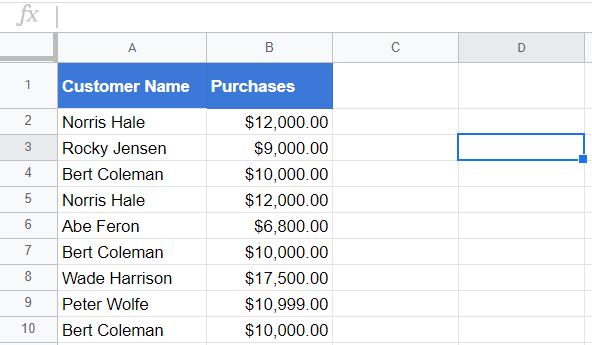
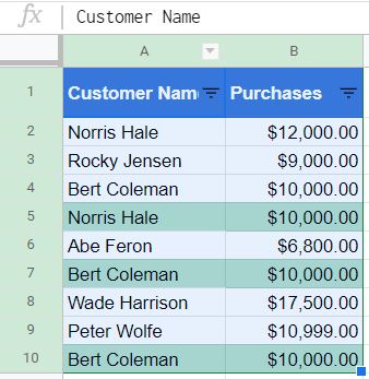
We have a spreadsheet that details the information of customers and their total purchases. The sheet reports purchases in United States Dollar (USD). We can observe duplicate entries in our sheet. We have highlighted the duplicates so that you could sort them out.

Now, these are just ten rows. You could have thousands or millions of rows that might contain duplicate records. That's why we need automated and quick methods to remove duplicates in Google Sheets.

How should we go about this problem?

We would use different methods for removing duplicates. After reading this article, you will be familiar with different ways of going about this problem.

How to Remove Duplicates in Google Sheets

Method 1: Removing Duplicates by Using the Remove Duplicates Feature

'Remove Duplicates' is a built-in feature in Google Sheets. It is present in the menu under Data > Remove Duplicates . It is super easy to use. We'll see how:

1. We will be using our customer purchases spreadsheet. It contains duplicate entries for customers, Norris Hale and Bert Coleman.

2. Before we move on to the Remove Duplicate feature, we'll select the data range. We would select all the data in our sheet. Right-click on cell A1 and drag the mouse across the rest of the cells.

3. The Remove Duplicates feature is built into Google Sheets. You need to navigate to the menu and click on Data > Remove Duplicates .

4. Once you've clicked on Remove Duplicates, you will see a menu pop up.

5. We'll check the Data has header row field. This will let the Google Sheets know about our header row. Otherwise, it would consider the first row as a data record.

6. We will keep the Select All option checked for now. Select all would consider both the columns, which in our case are columns A and B. In other words, it looks for the entire row and weeds out the duplicates. Proceed by clicking the Remove duplicates button.

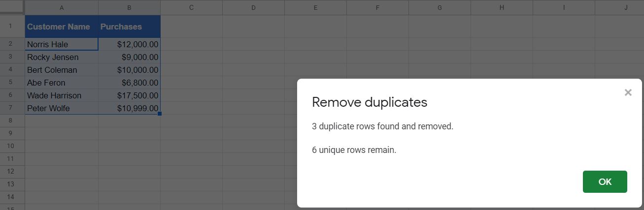
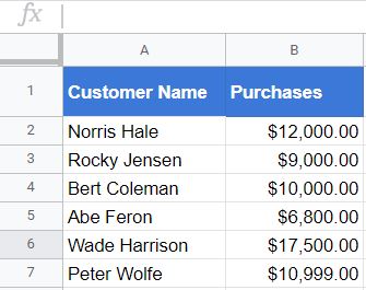
7. Google Sheets has successfully removed three duplicate rows, and now we are left with six unique values. Therefore, we have only one entry for Norris Hale and Bert Coleman.

8. However, sometimes we need to remove duplicates from a single column only, regardless of what values the duplicates might have in the other columns. To demonstrate this, we will go back to the original customer purchases spreadsheet. We will change the Purchases value from $10,000.00 to $9,000.00 for Bert Coleman entry in the seventh row.

9. Now if we repeat Steps 2 to 6 for this modified sheet, we get the following output.

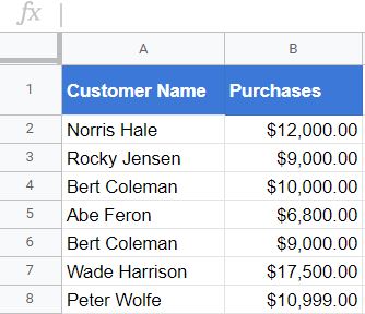
10. If we observe, we can see Bert Coleman is repeated twice. Why is that? That's because we have used Remove Duplicates for both the columns. So, it won't just consider Customer Name but also the Purchases entry. What if we want to remove duplicates regardless of the value in Purchases?

11. We'll restore the sheet given in Step 9 and perform Steps 2 and 3. Now, in the 'Remove duplicates' menu, let's uncheck the Select All and Column B – Purchases. We'll keep Column A- Customer Name checked. That's because we want to remove duplicate names regardless of their purchase values.

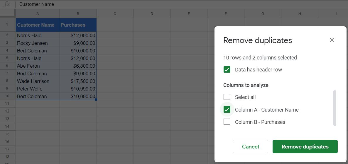
12. Click Remove Duplicates and you'll see that Google Sheets has removed all the duplicate names regardless of their purchase value.

We're done. We hope that you would be able to use the 'Remove Duplicates ' feature now. Let's move on to our next method.

Method 2: Removing Duplicates by Using Formulas

We can use different formulas to remove duplicates in our google sheet. We'll see the UNIQUE and COUNTIF. However, before you jump into the tutorial, you'll need to familiarize yourself with the syntax and working of both the functions.

Now, we've already covered the COUNTIF function in one of our articles, How to Use COUNTIF Function in Google Sheets . If you're not familiar with the function, this article can guide you well.

We'll understand the UNIQUE function and then move on to the tutorials.

The Anatomy of the UNIQUE Function in Google Sheets

The syntax of the UNIQUE function is as follows:

          =UNIQUE(range)        

• = is the equals sign that starts off any function in Google Sheets.
• UNIQUE is the name of our function.
• range is the array or range containing the dataset to consider.

The UNIQUE function discards the duplicates and returns the unique rows.

Removing Duplicates by Using UNIQUE Function

1. We will be using our customer purchases Google Sheet. It contains duplicate entries for customers, Norris Hale and Bert Coleman.

2. Click on a random cell outside this data range. Let's say we click on the cell D3.

3. We will enter the UNIQUE formula in this cell. We will start by typing '=' either directly in the cell or formula box above. Then we'll type the name of the function. We'll type ' (' right after it.

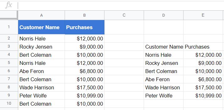
4. Now, we will select a range for the unique function. Let's say we need to check for duplicates rather than a single column. Therefore, we'll select the entire data range A1:B10.

5. Once we click Enter , we'll see that Google Sheets has created another table for us. This now doesn't contain duplicate entries.

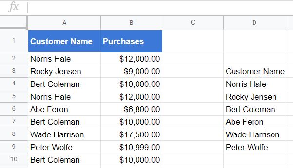
6. We can follow the same procedures for a single column as well. We'll repeat the Steps from 1 to 3. Now, for a single column, we will select a data range containing cells of that column. Let's say we want to remove duplicates from column A . We will enter the range as A1:A10 .

7. Press Enter . The output is data from column A with no duplicates.

That's it. We've learned how to use the UNIQUE function for removing duplicates. Now we'll move to another function: COUNTIF

Removing Duplicates by Using COUNTIF Function

We assume that you've already been familiar with this function. If not, you can learn about it by visiting the link given at the beginning of this section. We'll jump directly to the tutorial.

1. We will be using our customer purchases spreadsheet. It contains duplicate entries for customers, Norris Hale and Bert Coleman.

2. We will insert a column at C and name it Duplicates .

3. Let's say we want to remove duplicate rows rather than duplicates in a single column. We will type the following formula in column
   

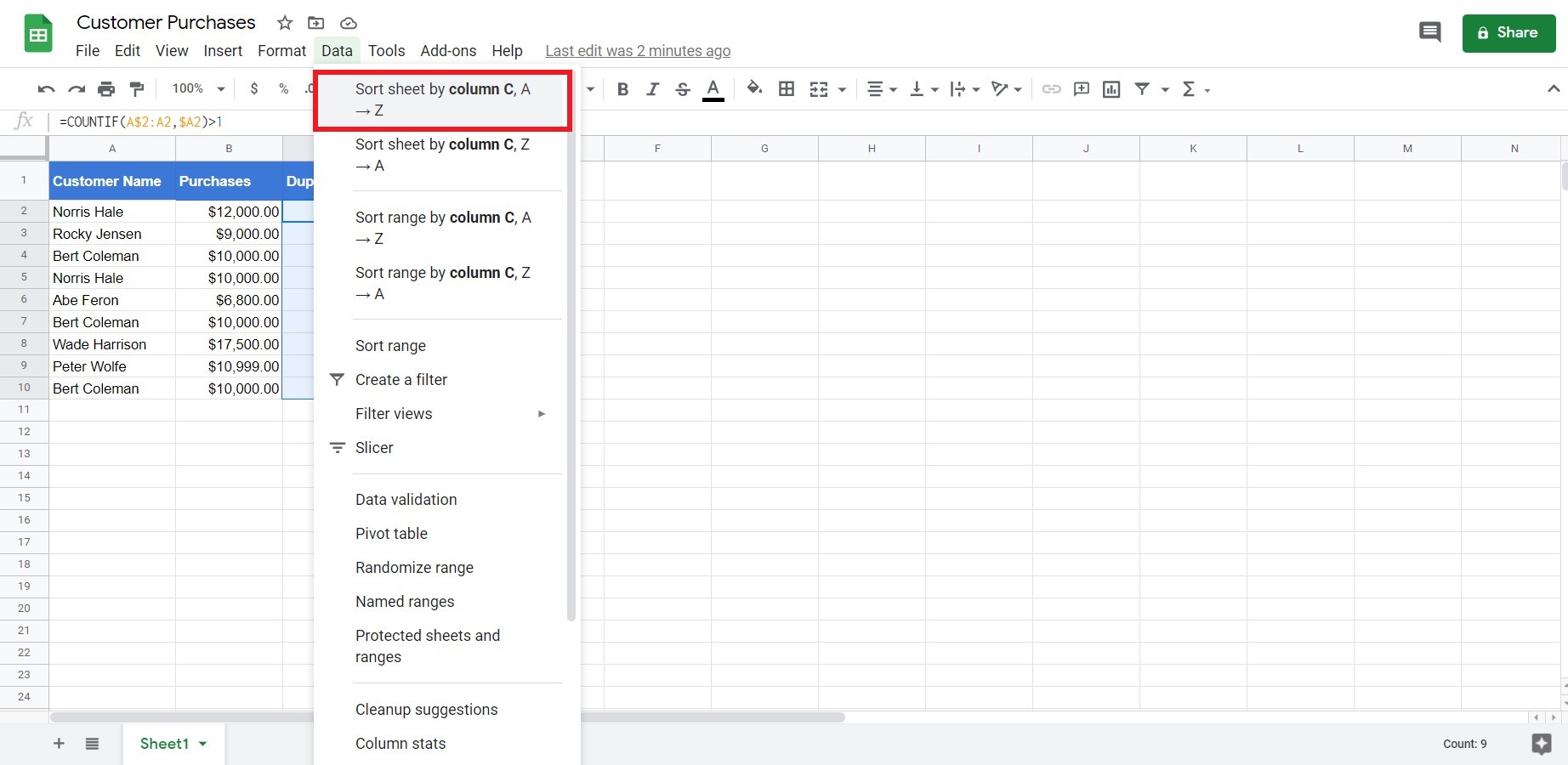
                 =COUNTIF(A$2:A2,A2)>1            

4. Press Enter and drag the response in cell C1 down to C10 . This can be done by right-clicking on the small blue square at the bottom-right of the cell C1 and then dragging it down to C10.

5. You will get the following output.

6. Select cells in the range C2:C10 .

7. Now, navigate to the top menu and select Data > Sort sheet by column C, A -> Z .

8. We get a sorted column where TRUE values are stacked at the bottom of the sheet.

9. As you might have noticed by now, column A of these rows contains duplicate values. We will select these rows as.

10. Click the Delete key on your keyboard to remove the duplicates. We're done.

We've seen how to remove duplicates in Google Sheets by using formulas. Now, we will move on to another method.

Method 3: Removing Duplicates by Using Conditional Formatting

Conditional formatting involves formatting cells based on a given formula. We'll use this method for removing the duplicates. However, you need to familiarize yourself with the COUNTIF function before reading the tutorial. We've already covered the COUNTIF function in one of our articles, " How to Use COUNTIF Function in Google Sheets " .

If you are familiar with the COUNTIF function, then let's jump straight into the tutorial.

1.  We will be using our customer purchases spreadsheet. It contains duplicate entries for customers, Norris Hale and Bert Coleman.

2. Before we move on to the Conditional Formatting , we'll select the data range. We would select all the data in our sheet. Right-click on cell A1 and drag your mouse across the rest of the cells.

3. To access Conditional Formatting, navigate to the menu, and click on Format > Conditional Formatting.

4. The Conditional Formatting menu then appears on the right side of the screen.

5. In this menu, we will click on the Format cells if 's drop-down.

6. From the Format cells if drop-down menu, we will navigate to Custom Formula is.

7. Once we have selected the Custom formula is , we'll see a value or formula entry box. We'll enter the following formula in it.
   

                 =COUNTIF($A$1:$A1,$A1)>1            

8. Click the Done button, afterward. You'll see that duplicate rows are highlighted in green. You can change the formatting using the Formatting style on the Conditional Formatting menu.

9. We can do this procedure for a single column as well. We will iterate the Steps from 1 to 6. Now we'll enter the formula with a slight modification. With this modification, now we can highlight a single row. We have done it for column A. Although, it can be done for any column.
   

                 =COUNTIF($A$1:$A1,A1)>1            

10. Click on the Done button and then we can see that it highlights duplicates from column A only.

11. Select cell A1 . Then navigate to the menu and select Data > Create a Filter .

12. The filter icon appears on the column headers.

13. Click on the filter icon present in the header cell. Then, from the drop-down select Filter by color > Fill Color > #B7E1CD. Although, the color code could vary depending on which color you've chosen for formatting.

14. Click OK and Google Sheets will filter out the highlighted values, which are the duplicate values.

15. Select all the rows and press the Delete key on your keyboard.

16.  Now navigate back to the menu and click on Data > Turn off Filter .

17. We have successfully removed the duplicate values. However, we now have empty rows instead.

18. To remove empty rows, we will select data in range A2:B9 . Then navigate to the menu and select Data > Sort range by Column B, A->Z .

19. Finally, we're done.

Quite a long method, but it can be used to remove duplicates for single as well as multiple columns.

Method 4: Removing Duplicates by Using Add-Ons

Add-ons are plugins that are developed by third-party developers. They could provide you extra functionalities that are not built into  Google Sheets. You can add them to your Google Sheets. There are many add-ons for different functions. However, we will download the one we are interested in.

In this tutorial, we will see how to download an add-on, and then we will use it to remove duplicates in our sheet.

1. We will be using our customer purchases spreadsheet. It contains duplicate entries for customers, Norris Hale and Bert Coleman.

2. To download an add-on, we will navigate to the menu and select Add-ons > Get add-ons.

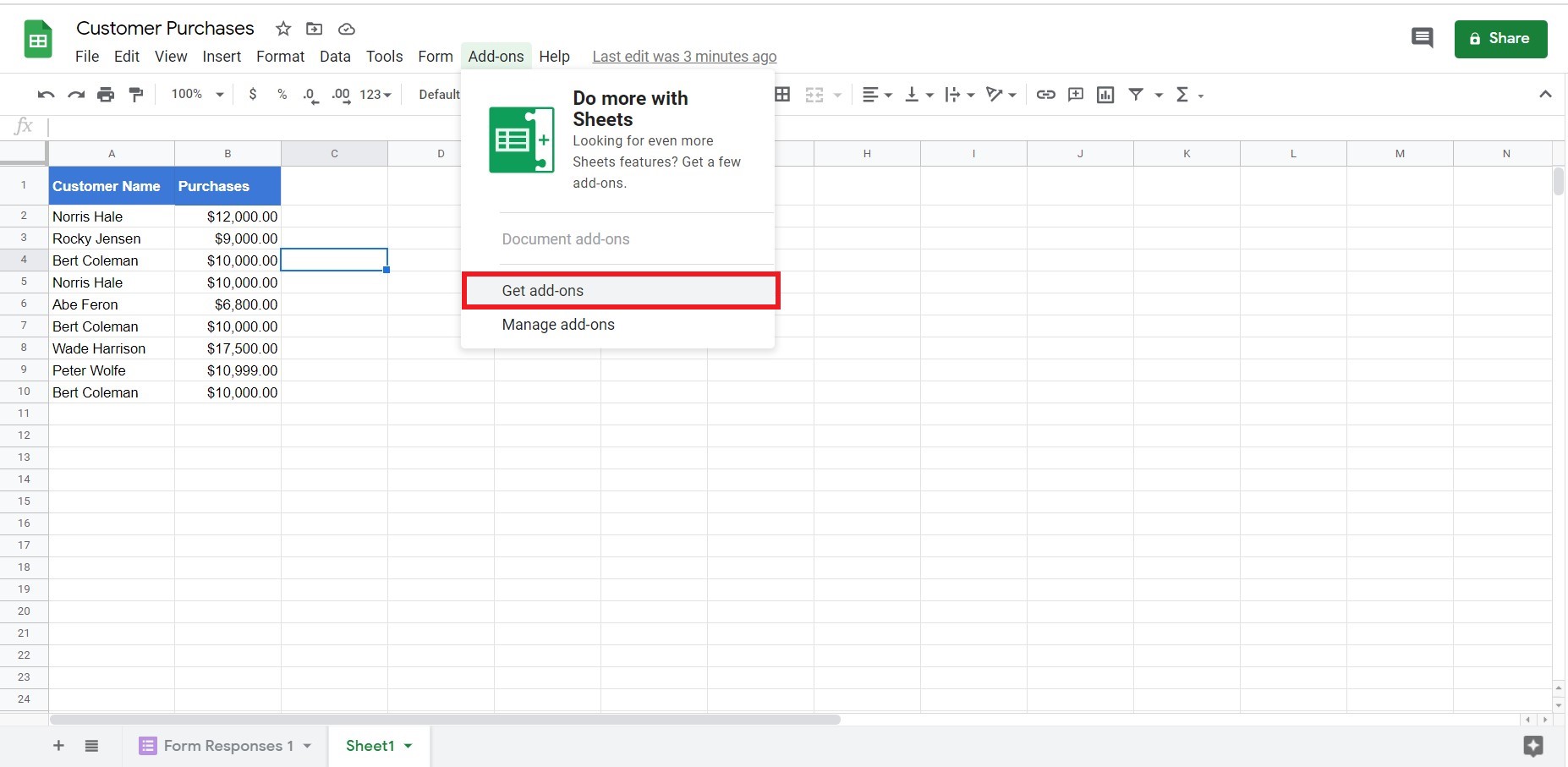
3. The Add-ons menu will pop up.

4. In the Search apps , type the keyword Remove Duplicates and press Enter. The Add-ons menu will then show the relevant add-ons.

5. We will download the first add-on from the left.

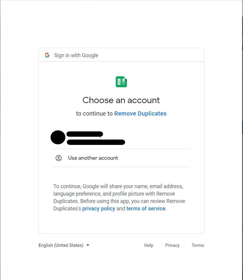
6. We click on it and it will take us to the download menu. There, we will click on the Install button. Then, it will require you to select your Gmail account and log in if you're not.

7. Once you download this, it will be added to the Add-ons drop-down menu. We can access it from the menu by selecting Add-ons > Remove Duplicates > Find duplicate or unique rows .

8. Upon clicking this, we will be redirected to the Find duplicate and unique rows menu . There we will select the range of data. Let's select the full data range from A1:B10 .

9. Clicking on the Next > button will redirect us to yet another menu. This menu offers different options for working with duplicate and unique data. However, we will select the first option.

10. Clicking on next will take us to the menu where we could select the columns that we would like to find duplicates in. We'll select both the columns.

11. Click the Next button to proceed to the final menu. Here we could select different options based on what we want to do with duplicate values. However, we will select Delete rows within selection option.

12. Click Finish and you're done. Voila!

So far so good. We have seen how to remove duplicates in Google Sheets using four different methods. You could pick any one of these methods based on your requirements and preference.

That should be all you need. You can now remove duplicates in Google Sheets. Check out our other numerous Google Sheets formulas to create even more complex and useful functions in Google Sheets.

Get emails from us about Google Sheets.

Our goal this year is to create lots of rich, bite-sized tutorials for Google Sheets users like you. If you liked this one, you'll love what we are working on! Readers receive ✨ early access ✨ to new content.

how to delete duplicates in google sheets

Source: https://www.sheetaki.com/remove-duplicates-in-google-sheets/

Posted by: jankowskiinteall.blogspot.com

Share this post